12  Compartmental models

Author
Affiliation

Nik Cunniffe

University of Cambridge

Understanding plant disease epidemics requires more than simply describing patterns of spread. Models which represent the biological processes generating those patterns are more informative.

Process-based models do exactly this, by explicitly linking epidemiological dynamics to underlying mechanisms such as transmission and latent infection (Madden et al. 2007). This provides a framework for interpreting observations, predicting epidemic behaviour and evaluating the likely impact of control strategies.

The dominant paradigm is compartmental modelling, an approach also widely used for diseases of animals and humans (Keeling and Rohani 2008). In this framework, the host population is divided into a set of mutually exclusive classes (“compartments”) based on disease status, with epidemic dynamics represented by the movement of hosts between compartments. For plant diseases, the basic concept goes at least as far back as the seminal work of van der Plank (1963). This simple idea provides a flexible and extensible structure for modelling a wide range of epidemiological systems.

In plant disease, the appropriate choice of unit that is represented by the compartments depends on the biological context (Cunniffe and Gilligan 2020). For systemic pathogens, such as viruses or some bacteria, it can often be natural to treat individual plants as the fundamental unit. For many diseases, however, and particularly for fungal diseases, infection occurs at much finer scales. Models of these diseases therefore typically instead focus on tissues such as leaves or roots, or even smaller infectable sites (e.g., sections of a leaf which could support a single lesion). At the other extreme, compartmental models can also be used to track disease at much larger spatial scales, for example by taking the quantum to be fields, farms or regions. Such scale-invariance is one of the major strengths of the approach (Madden 2025).

Beyond their role in representing biological processes, compartmental models are particularly valuable because they form a coherent framework within which the epidemiological impacts of additional complexity can be incorporated and assessed. Biology such as host growth, seasonal cropping cycles, environmental drivers, vectored spread, time-dependent rates, interactions between diseases and disease management interventions can all be introduced by modifying the structure of compartments or the rates of transition between them. Parameters in the model have biological meanings, which allows us to understand and distinguish how different processes affect the epidemiology.

This flexibility is particularly important in plant disease systems, where epidemics often unfold across multiple spatial and temporal scales, and where management decisions must account for both short-term dynamics and longer-term persistence.

As a result, compartmental models are not simply abstract descriptions of epidemics, but practical tools for linking biological understanding to decision-making in real plant disease systems.

In this chapter, we develop this framework progressively. We begin by constructing a simple within-season model, explore its behaviour and key epidemiological properties, and then extend it step by step to incorporate additional biological realism, including primary infection, host growth and multi-season dynamics. Along the way, we show how these models can be implemented and explored using R.

12.1 A starting point: the H-L-I-R model

We begin with the simplest useful compartmental model which tracks an epidemic within a single growing season. This serves as a foundation that we will later extend to more complex biological situations.

12.1.1 Biological basis of the model

The key epidemiological difference between individual diseased hosts or units of host tissue is infection status: pre-infectious, infectious or post-infectious. The most obvious compartmental model therefore tracks these three classes of diseased hosts, together with an additional compartment for uninfected healthy hosts.

In plant disease modelling, this formulation is often referred to as the H-L-I-R (Healthy-Latent-Infectious-Removed) model (Madden et al. 2007). This terminology can obscure the close relationship with the extensive literature on S-E-I-R (Susceptible-Exposed-Infected-Removed) models (Keeling and Rohani 2008), which are based on precisely the same epidemiological reasoning.

12.1.2 Specifying the model

To construct the model, we first describe the biological processes governing transitions between compartments using word equations, before translating these into mathematical form.

The rates of change are

\[ \small \begin{aligned} \mbox{Rate of change of healthy hosts} &= -\mbox{Infection},\\ \mbox{Rate of change of latently infected hosts} &= \mbox{Infection} - \mbox{Emergence of infectivity},\\ \mbox{Rate of change of infectious hosts} &= \mbox{Emergence of infectivity} - \mbox{Loss of infectivity},\\ \mbox{Rate of change of removed hosts} &= \mbox{Loss of infectivity}. \end{aligned} \]

Schematic showing the H-L-I-R compartmental model. The arrows represent the three transitions tracked by the model: infection, emergence of infectivity and loss of infectivity. The dashed line linking the \(I\) compartment to the infection transition indicates the rate of this transition depends on the value of \(I\) (as well as the value of \(H\)).

Transitions come in pairs, since movement between a pair of compartments is being tracked. For example, the Infection transition causes hosts to change status (“move”) from the healthy compartment to the latently infected compartment.

Specifying the model requires us to be more precise about the rates of the three transitions. It is intuitive that, all other things being equal, the net rate at which hosts enter the infectious compartment (the \(L \rightarrow I\) transition) should depend only on the number of latently infected hosts. Similarly, the net rate at which infectious hosts are removed (the \(I \rightarrow R\) transition) depends only on the number of infectious hosts.

In both cases, rates of these transitions are therefore proportional to the number of hosts which could potentially make the transition, with

\[ \small \begin{aligned} \mbox{Net rate of emergence of infectivity} &\propto \mbox{Number of latently infected hosts},\\ \mbox{Net rate of loss of infectivity} &\propto \mbox{Number of infectious hosts}.\\ \end{aligned} \]

The rate at which hosts become latently infected (the \(H \rightarrow L\) transition) is more complex. It depends on the current number of healthy hosts, since an individual host can only first become latently infected once. However, since infection is driven by spread from infectious hosts, the rate of the transition should also depend on the number of infectious hosts.

The simplest assumption is to assume bilinearity, i.e., to assume that the rate depends on the product of the number of healthy and infectious hosts. This is sometimes called “mass-action” transmission, and corresponds to homogeneous mixing of hosts, i.e., inoculum from any infectious host is equally likely to cause infection of any other host.

A word equation for the transition rate corresponding to infection is

\[ \small \begin{aligned} \mbox{Net rate of infection} &\propto \mbox{Number of healthy hosts} \times \mbox{Number of infected hosts}.\\ \end{aligned} \]

Finally, note that the interpretation of the removed compartment depends on the biological system. In some pathosystems it may correspond to dead hosts, in others to hosts that remain diseased but are no longer infectious, and in yet others to hosts that have been harvested or otherwise removed from disease transmission. The key feature is that individuals in the removed compartment no longer contribute to new infections.

12.1.3 Writing the model as a system of differential equations

Having specified the transition processes, we can now express the model formally.

State variables in the H-L-I-R model.
Symbol Meaning
\(H(t)\) Healthy hosts at time t
\(L(t)\) Latently infected hosts at time t
\(I(t)\) Infectious hosts at time t
\(R(t)\) Removed hosts at time t

If we introduce the following symbols for parameters

  • \(\gamma\) = rate at which latently infected hosts become infectious (per unit time)
  • \(\mu\) = rate at which infectious hosts lose infectivity (per unit time)
  • \(\beta\) = rate of infection (per unit time, per infected host, per healthy host)

then the H-L-I-R model can be expressed as a system of differential equations

\[\begin{aligned} \frac{dH}{dt} &= -\beta I H,\\ \frac{dL}{dt} &= \beta I H - \gamma L,\\ \frac{dI}{dt} &= \gamma L - \mu I,\\ \frac{dR}{dt} &= \mu I. \end{aligned}\]

12.1.4 Numbers versus proportions

We have chosen to model the numbers of hosts in each compartment, so that

\[H+L+I+R=N,\]

where \(N\) is the total host population size.

An alternative formulation is to model the corresponding proportions

\[h = H/N,\quad l = L/N,\quad i = I/N,\quad r = R/N,\]

which satisfy

\[h+l+i+r=1.\]

Both approaches contain exactly the same epidemiological information. The choice is largely one of convenience.

Working with numbers can be helpful because it keeps the biological interpretation of the state variables very direct. However, formulations based on proportions are also common, particularly when comparing epidemics in populations of different sizes.

For example, dividing the H-L-I-R equations by \(N\) leads to

\[\frac{dh}{dt} = -\beta N i h,\]

with analogous equations for the other compartments. In this formulation, the epidemiologically important quantity is often the product \(\beta N\), rather than \(\beta\) itself.

The important message is that the numbers and proportions formulations contain exactly the same epidemiological information; only the interpretation of the parameters changes.

12.1.5 Meaning of the parameters

Interpreting the parameters biologically connects the mathematical formulation back to observable processes in real systems.

For the per capita rates, \(\gamma\) and \(\mu\), there is a well-known inverse relationship between the rate at which an epidemiological event occurs and the time taken on average for the event to occur (Keeling and Rohani 2008). Here, this means that hosts are latently infected for \(1/\gamma\) time units, and the infectious period is \(1/\mu\) time units. Consequently, these parameters can be estimated from biological knowledge of the pathogen, for example based upon experiments which involve single hosts in isolation, without tracking interactions or epidemic behaviour.

Conversely, because the infection rate \(\beta\) combines inoculum production, dispersal, host contact and infection efficiency, it is generally not directly measurable in a simple experiment. Moreover, its value depends on factors such as host density, spatial scale and environmental conditions. Consequently, \(\beta\) is usually estimated by fitting models to epidemic data (see below).

As an aside, note it can sometimes be useful to partition \(\beta\) into its constituent parts, for example as \(\beta = \sigma \theta\), where \(\sigma\) relates to the susceptibility of healthy hosts, and \(\theta\) to the infectivity of infected hosts. For simple models this is largely a matter of presentation, since only the product ever appears in any mathematical expressions. However, making this distinction can be necessary when models are more complex, e.g., when they track pathogen spread on multiple host species with different epidemiological properties (Del Ponte et al. 2026).

12.1.6 Note on host demography

It is helpful to note an important simplifying assumption of the model as currently formulated.

For some pathogens the \(I \rightarrow R\) transition corresponds to disease-induced host death, i.e., the pathogen killing a host. It can also often be the case that the host has its own demography, e.g., there is natural production and/or death of hosts.

However, in the model as written above, natural host demography is ignored, i.e., hosts only change status by moving from one epidemiological compartment to the next, with no production of new healthy tissue or (natural) death.

We can see mathematically that the total host population size, \(N = H + L + I + R\), is constant in our model by noting \[\frac{dN}{dt} = \frac{dH}{dt} + \frac{dL}{dt} + \frac{dI}{dt} + \frac{dR}{dt} = 0.\] This is because all transitions between compartments come in pairs, with all outflows from a compartment matched by a corresponding inflow to another compartment.

We show later how within-season growth of hosts can be included in the model.

Symbols and parameters used throughout this chapter. State variables are quantities whose values change over time. User-specified parameters determine the rates at which these changes occur. In practical applications, some parameters may be known from biological experiments, while others must be estimated by fitting the model to epidemic data (see below).
Symbol Meaning Type/Definition
\(H(t)\) Number of healthy hosts at time \(t\) State variable
\(L(t)\) Number of latent hosts at time \(t\) State variable
\(I(t)\) Number of infectious hosts at time \(t\) State variable
\(R(t)\) Number of removed hosts at time \(t\) State variable
\(P(t)\) Density of primary inoculum at time \(t\) State variable
\(t\) Time Independent variable
\(\alpha\) Primary infection rate User-specified parameter
\(\beta\) Secondary infection rate User-specified parameter
\(\gamma\) Rate at which latent hosts become infectious User-specified parameter
\(\mu\) Rate at which infectious hosts become removed User-specified parameter
\(\omega\) Rate of decay of primary inoculum User-specified parameter
\(r_H\) Host production rate User-specified parameter
\(N\) Fixed total host population size in the basic H-L-I-R model \(N = H + L + I + R\) (constant)
\(T(t)\) Total number of hosts when host growth is included \(T(t) = H(t) + L(t) + I(t) + R(t)\)
\(D(t)\) Total number of diseased (i.e., non-healthy) hosts \(D(t) = L(t) + I(t) + R(t)\)
\(N_{max}\) Carrying capacity User-specified parameter
\(T_{\max}\) Length of growing season User-specified parameter
\(\phi\) Inoculum production rate User-specified parameter

12.1.7 Assumptions underpinning the H-L-I-R model

Like all mathematical models, the H-L-I-R model is a simplified representation of reality. Its value lies not in reproducing every biological detail, but in capturing the dominant processes driving epidemic behaviour. Understanding the assumptions of the model is therefore probably just as important as understanding the equations themselves.

The H-L-I-R model makes the following assumptions:

  • Homogeneous mixing. Every infectious host is assumed to be equally likely to infect every healthy host. The infection rate therefore depends on the product \(IH\). This may be reasonable in well-mixed systems, but becomes less appropriate when spatial structure or local dispersal is important.

  • Identical hosts. All hosts are assumed to be epidemiologically identical. The model does not distinguish between resistant and susceptible cultivars, young and old hosts, or hosts experiencing different environmental conditions.

  • Fixed parameter values. The transmission rate (\(\beta\)), latent period (\(1/\gamma\)) and infectious period (\(1/\mu\)) are assumed constant throughout the epidemic. In reality these quantities often vary with weather, host development stage and management actions.

  • Deterministic dynamics. The model predicts the average epidemic trajectory and ignores random events. Consequently, if \(R_0 > 1\) (see below), invasion always occurs in the model, whereas chance extinction may occur in real epidemics when infection levels are low.

  • Continuous time. Hosts move continuously between epidemiological states. This is usually a good approximation when populations are large, although some biological processes may occur at more discrete intervals.

  • Closed population. No hosts enter or leave the system. As described above, the total host population therefore remains constant, and so the model excludes host growth, harvesting and natural host mortality.

Much of the remainder of this chapter can be viewed as a sequence of examples of progressively relaxing these assumptions. Adding primary inoculum relaxes the assumption of a closed epidemic system. Adding host growth relaxes the assumption of a fixed host population. Extending to multiple seasons relaxes the assumption that epidemics begin and end within a single growing season.

12.2 Exploring the model through simulation

12.2.1 Solving the H-L-I-R model numerically

To solve the model numerically, we use the deSolve library in R.

To do this, we must specify the numerical values of the parameters; here we take these to be

  • \(\beta = 0.00003\) host\(^{-1}\) day\(^{-1}\)
  • \(\gamma = 0.2\) day\(^{-1}\)
  • \(\mu = 0.1\) day\(^{-1}\)

Note that since we have cast the model in terms of numbers of hosts, \(\gamma\) and \(\mu\) have units day\(^{-1}\), whereas \(\beta\) has units per host per day. This is why the product \(\beta N\), rather than \(\beta\) alone, appears in expressions such as \(R_0\) (see below) or in the equivalent proportion-based formulation.

Given the inverse relationships described above, the choice of \(\gamma\) corresponds to a pathogen with a \(5\) day latent period, and the choice of \(\mu\) means the infectious period is \(10\) days.

Numerical solution also requires initial conditions. We assume there is a single latently infected host in a population of size \(N = 10000\), which means

  • \(H(0) = 9999\)
  • \(L(0) = 1\)
  • \(I(0) = 0\)
  • \(R(0) = 0\)

The final component is specifying the range of time over which we are interested in knowing the solution. Here we take \(0 \le t \le T_{max} = 250\) (days), corresponding to a \(250\)-day period.

The key computational step is the call to the function deSolve::ode(), which requires the caller to specify four arguments

  • initial condition (hlir.init)
  • set of times for which a solution is required (hlir.time)
  • right-hand side of the system of differential equations (hlir.model)
  • parameters to the system of differential equations (hlir.params).

The syntax, perhaps particularly the way parameters are handled by the function hlir.model, is somewhat arcane. However, as we shall see, this code provides a template which can, in principle, readily be adapted to any system.

library(deSolve)

# specify the model via a function encoding the right hand side
hlir.model <- function(t, state, parameters) {
  with(as.list(c(state, parameters)), {
    dH <- - beta * I * H
    dL <- beta * I * H - gamma * L
    dI <- gamma * L - mu * I
    dR <- mu * I
    list(c(dH, dL, dI, dR))
  })
}

# Specify parameters
N <- 10000
T.max <- 250

hlir.params <- c(beta = 0.00003, 
                 gamma = 0.2, 
                 mu = 0.1)

# Specify initial conditions
hlir.init <- c(H = N - 1, 
               L = 1, 
               I = 0, 
               R = 0)

# Specify range of times for which a solution is required
hlir.time <- seq(0, T.max, by = 0.01)

# Solve the model
hlir.sol <- ode(y = hlir.init, 
                times = hlir.time, 
                func = hlir.model, 
                parms = hlir.params)

# Cast results to a R data frame
hlir.sol.df <- data.frame(hlir.sol)

# Plot results using our custom helper function
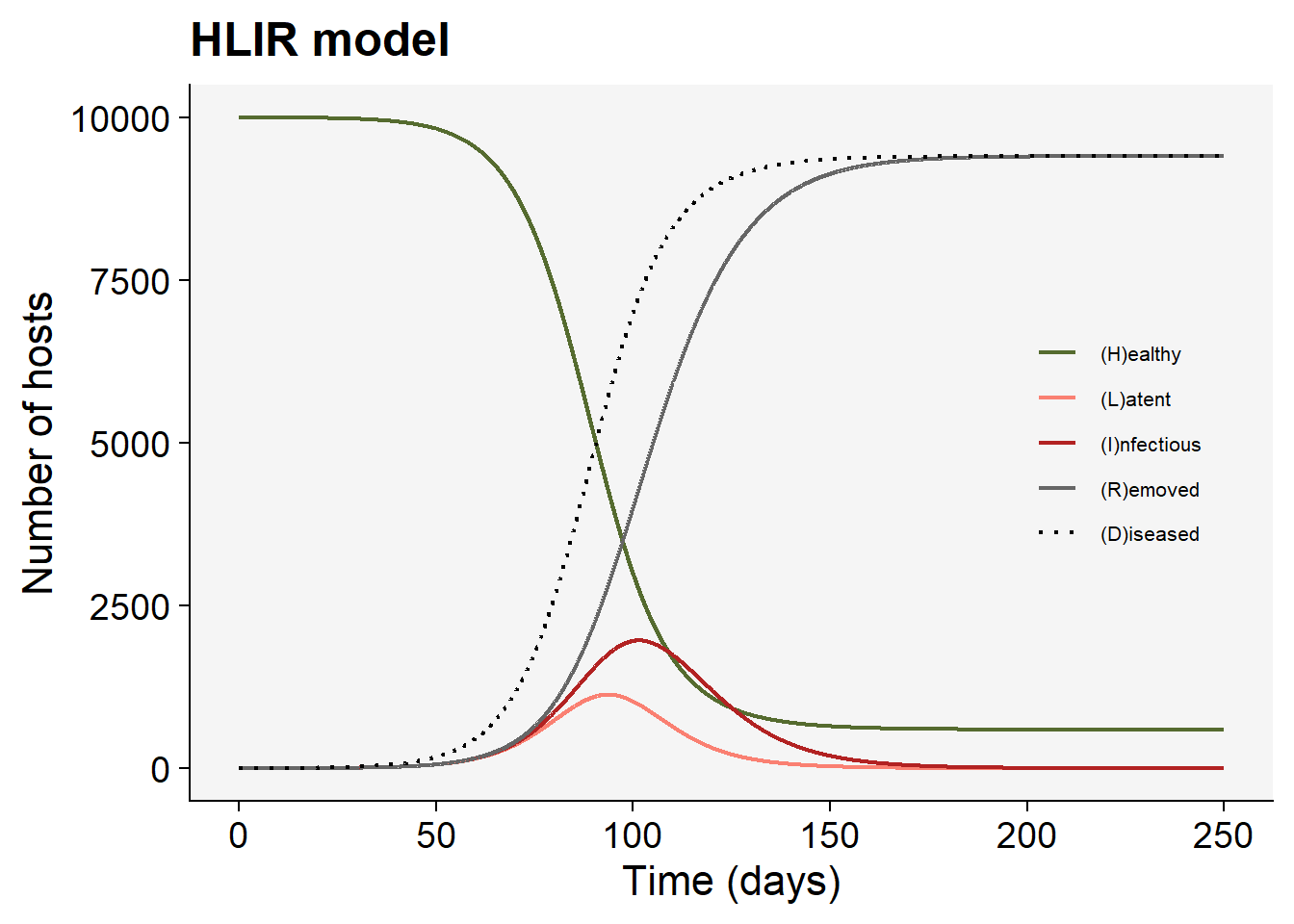
plot.model.results(hlir.sol.df, type="HLIR")

12.2.2 Interpreting epidemic behaviour

The simulation shows the characteristic behaviour of an epidemic. Initially, disease prevalence increases slowly, but then the epidemic accelerates, causing a rapid decline in healthy hosts. Eventually, depletion of healthy hosts limits transmission and the epidemic dies out, with most (but not all) hosts entering the removed class.

The key features to notice are the lag before infectious tissue builds up, the subsequent rapid loss of healthy hosts, and the eventual plateau in total diseased tissue.

The number of diseased hosts, \(D(t)\), is also shown, where \[\begin{align} D(t) &= L(t) + I(t) + R(t). \end{align}\]

While numerical simulation provides a detailed picture of epidemic behaviour, it is often useful to summarise these dynamics using a small number of quantitative measures.

In particular, we may wish to answer questions such as:

  • Under what conditions can an epidemic invade?
  • How large will the epidemic become?
  • How quickly will infection spread initially?

Compartmental models allow these questions to be answered analytically through a set of standard epidemiological quantities and calculations, which we now introduce.

12.3 Key epidemiological quantities

Certain calculations are routine using compartmental models, and provide concise summaries of key features of epidemic dynamics. We illustrate these for the H-L-I-R model here.

12.3.1 Basic reproduction number

The first question is whether a pathogen can successfully invade a healthy host population.

In the H-L-I-R model an individual host’s infectious period is finite and therefore a pathogen cannot invade if its net rate of infection is too low relative to how long it stays infectious.

This important idea is captured in a key threshold, the basic reproduction number, \(R_0\), the number of new infections resulting from the introduction of a single infected host into an otherwise healthy population.

There are a number of methods of different levels of mathematical sophistication for finding \(R_0\). For simple models, it can be found heuristically.

Assuming the total size of the population is \[H + L + I + R = N,\] then at the start of a potential epidemic initiated by a single infected host, \[L = R = 0,\] and \[I = 1,\] and \[H = N - 1\approx N.\]

Considering only the infections directly caused by the single infected host and multiplying the net rate at which healthy hosts become infected by the host’s average infectious period implies \[\begin{align} R_0 &= \mbox{Rate of infection per healthy host} \times \mbox{Number of healthy hosts} \times \mbox{Infectious period},\\ &\approx \beta \times N \times \frac{1}{\mu},\\ &= \frac{\beta N}{\mu}. \end{align}\] This is because the infected host generates infections at total rate \(\beta N\) and remains infectious for \(1/\mu\) time units.

If \(R_0 > 1\) then the pathogen will invade and the amount of infection will increase over time, at least initially.

Note that the parameter controlling the rate of emergence of infectivity (\(\gamma\)) is not involved in the expression for \(R_0\), i.e., the pathogen’s basic reproduction number is independent of its latent period. This makes sense, because in this model the latent period only affects how rapidly hosts are infected, rather than how many infections are caused. Note this would no longer be true if natural death were included in the model, since then we would need to account for the probability of a latently infected host successfully becoming infectious rather than dying naturally. In the current model, although hosts spend time in the latent compartment before becoming infectious, every latently infected host is guaranteed to eventually reach the infectious compartment. The latent period therefore alters the timing of transmission but not the number of secondary infections generated.

For this parameterisation of the H-L-I-R model, \(R_0 = 3\).

hlir.r0.func <- function(beta,N,mu)
{
  return(beta * N / mu)
}

hlir.r0 <- hlir.r0.func(hlir.params[["beta"]],
                        N,
                        hlir.params[["mu"]])
              
print(paste("R0 =",hlir.r0))
[1] "R0 = 3"

12.3.2 Final size equation

While \(R_0\) determines whether an epidemic can invade, it does not tell us how large the epidemic will become once it is established.

Not all hosts necessarily become infected by the end of the epidemic. This can be quantified by the final size equation (Keeling and Rohani 2008), which states that the fraction of the population which eventually becomes infected, i.e., \[f = 1 - H(\infty)/N\] satisfies \[f = 1 - \exp(-f R_0).\] Note that because in this model at the end of the epidemic \(L(\infty) = I(\infty) = 0\), all infected hosts are ultimately found in the removed compartment, and so \[f = R(\infty) / N.\]

The final size equation is a transcendental equation, and so must be solved numerically.

The code below uses the base R function uniroot to solve it in R, and compares this with the final value of \(R\) as obtained from the numerical solution at \(t = T_{max} = 250\) days.

hlir.final.size <- function(r0)
{
  f <- function(z) z - (1 - exp(-r0 * z))

  ret.val <- 0
  if(r0 > 1)
  {
    ret.val <- uniroot(f, lower = 1e-10, upper = 1)$root
  }
  return(ret.val)
}

hlir.f <- hlir.final.size(hlir.r0)
print(paste("From final size equation: f =", hlir.f))
[1] "From final size equation: f = 0.940479945459519"
print(paste("From numerical solution: f =", hlir.sol.df[which.max(hlir.sol.df$time), "R"]/N))
[1] "From numerical solution: f = 0.940466373627096"

In both cases, approximately 94% of all hosts are infected by the end of the epidemic, with a very small discrepancy between the two calculations because the epidemic has not quite completed within \(T_{max} = 250\) days.

12.3.3 Initial rate of epidemic increase

A complementary question concerns the speed of epidemic growth during the early stages of spread.

When disease is rare, almost all hosts are healthy, so the epidemic is operating near the disease-free equilibrium. In this regime, the nonlinear model behaves approximately like a linear system. The dominant behaviour of that linear system determines whether infection grows or declines, and how rapidly this occurs. The quantity \(r\) is the corresponding exponential growth rate.

This initial exponential rate of disease increase can be found (Cunniffe et al. 2012) by calculating the largest real part of the eigenvalues of the Jacobian matrix of the system evaluated at the disease-free-equilibrium \[(H,L,I,R)=(N,0,0,0)\] The Jacobian matrix is simply a mathematical object that captures how small perturbations to each compartment affect the rates of change of all other compartments.

This can be done using the function jacobian.full() in the rootSolve package.

library(rootSolve)

# disease free equilibrium
hlir.dfe <- c(H = N, 
              L = 0, 
              I = 0, 
              R = 0)

# find jacobian matrix at hlir.dfe
hlir.jac <- jacobian.full(y = hlir.dfe, 
                          func = hlir.model,
                          parms = hlir.params)

# find eigenvalues and eigenvectors
hlir.eigen.jac <- eigen(hlir.jac)

# extract and print the largest eigenvalue
print(paste("r =",max(hlir.eigen.jac[["values"]])))
[1] "r = 0.1"

Note that the calculation done by the code above involving the function rootSolve::jacobian.full() would in fact be the same for any compartmental model, and so does not require any mathematics. You do not need to understand the linear algebra here. The software does the calculation automatically.

That the numerical solution matches these theoretical expectations can be checked.

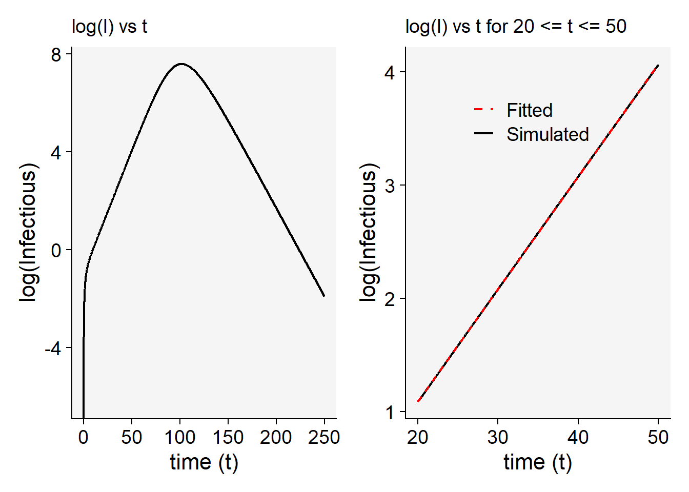
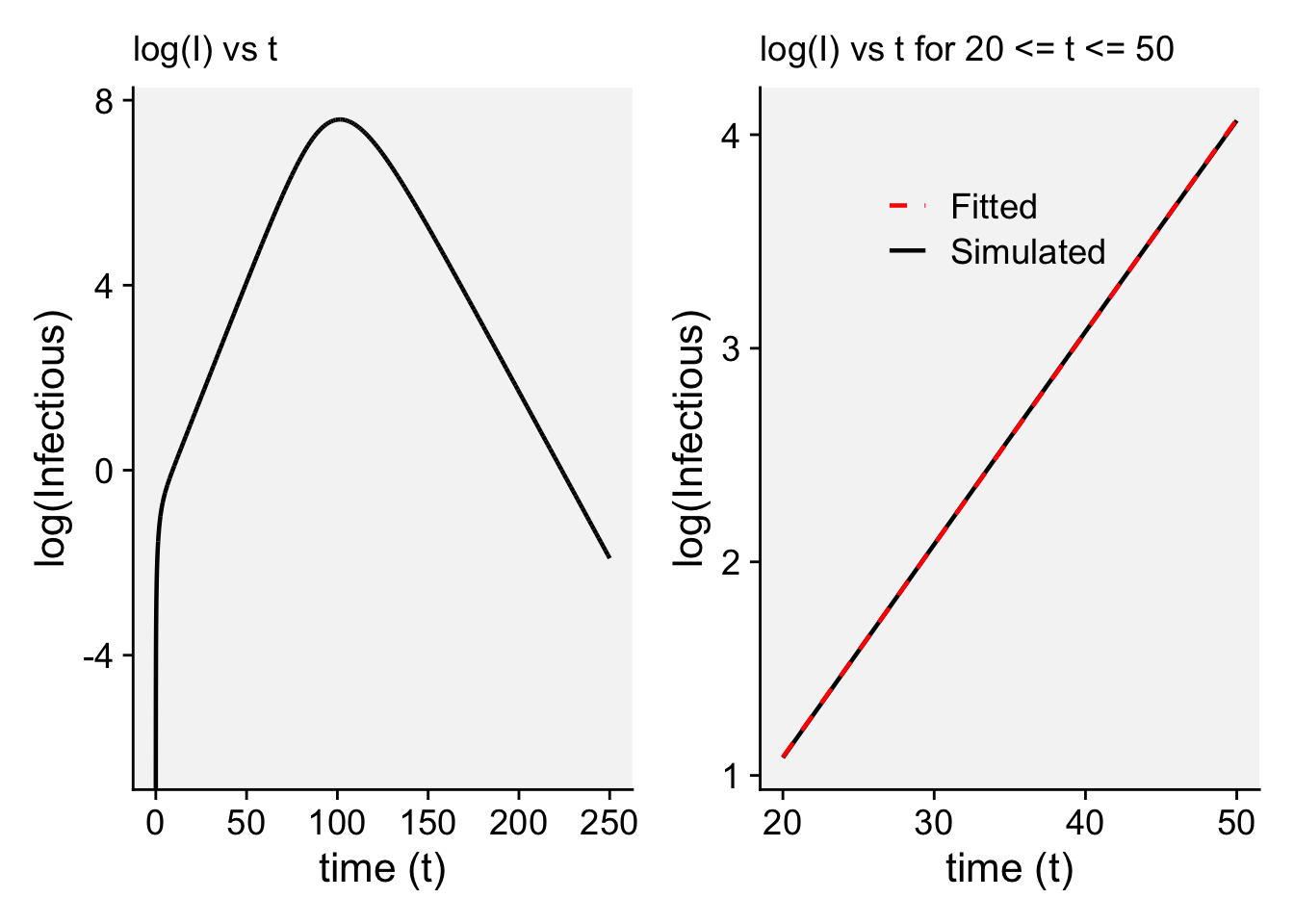
On the figures below, the left hand panel shows the logarithm of the number of infectious hosts as a function of time. There is an initial transient (for very small values of \(t\)) followed by an extended period (from around 10 to 100 days) within which the logarithm of the number of infectious hosts grows linearly, and so in which the number of infectious hosts is growing exponentially.

(Arbitrarily) selecting \(t_{start} = 20 \le t \le 50 = t_{end}\) as a representative region within this range of plausibly exponential increase, a subset of the curve is plotted on the right-hand side (black), together with the results of a linear regression (red).

library(ggplot2)
library(r4pde)
library(patchwork)
Warning: package 'patchwork' was built under R version 4.4.1
# First plot: log(I) vs t
p1 <- ggplot(hlir.sol.df, aes(x = time, y = log(I))) +
  geom_line(linewidth = 0.8) +
  labs(
    x = "time (t)",
    y = "log(Infectious)",
    subtitle = "log(I) vs t"
  ) +
  theme_r4pde()

# extract just t and I for 20 <= t <= 50
t.start <- 20
t.end <- 50
t.subset <- hlir.sol.df$time[hlir.sol.df$time>=t.start&hlir.sol.df$time<=t.end]
i.subset <- hlir.sol.df$I[hlir.sol.df$time>=t.start&hlir.sol.df$time<=t.end]

subset_df <- data.frame(
  time = t.subset,
  log_I = log(i.subset)
)

# fit a linear model and report its gradient
my.mod <- lm(log(i.subset)~t.subset)
print(paste("Fitted r =", coef(my.mod)[[2]]))
[1] "Fitted r = 0.0995145118548592"
# Predict values for the regression line
subset_df$pred <- predict(my.mod)

# Second plot: subset with regression line
p2 <- ggplot(subset_df, aes(x = time)) +
  geom_line(aes(y = log_I, color = "Simulated"), linewidth = 0.8) +
  geom_line(aes(y = pred, color = "Fitted"), linetype = "dashed", linewidth = 0.8) +
  scale_color_manual(
    name = NULL,
    values = c("Simulated" = "black", "Fitted" = "red")
  ) +
  labs(
    x = "time (t)",
    y = "log(Infectious)",
    subtitle = paste("log(I) vs t for", t.start, "<= t <=", t.end)
  ) +
  theme_r4pde() +
  theme(legend.position = c(0.25, 0.8))

p1 + p2

Note the initial exponential growth rate matches to two significant figures.

Together, these quantities — \(R_0\), the final size, and the initial growth rate — provide complementary summaries of epidemic behaviour, linking the structure of the model to biologically meaningful outcomes.

Although both \(R_0\) and \(r\) describe epidemic invasion, they capture different aspects of epidemic behaviour. \(R_0\) measures how many secondary infections are generated, whereas \(r\) measures how rapidly infection increases through time.

12.4 Extending the H-L-I-R framework: adding biological realism

12.4.1 Adding primary infection (H-L-I-R-(P) model)

To illustrate the flexibility of the compartmental framework, as well as to introduce further biology which will be needed to model multi-seasonal epidemics, primary infection is added to the model. This corresponds to infections caused by inoculum produced elsewhere (i.e., infections which are not direct secondary infections from infected hosts within the system of interest)

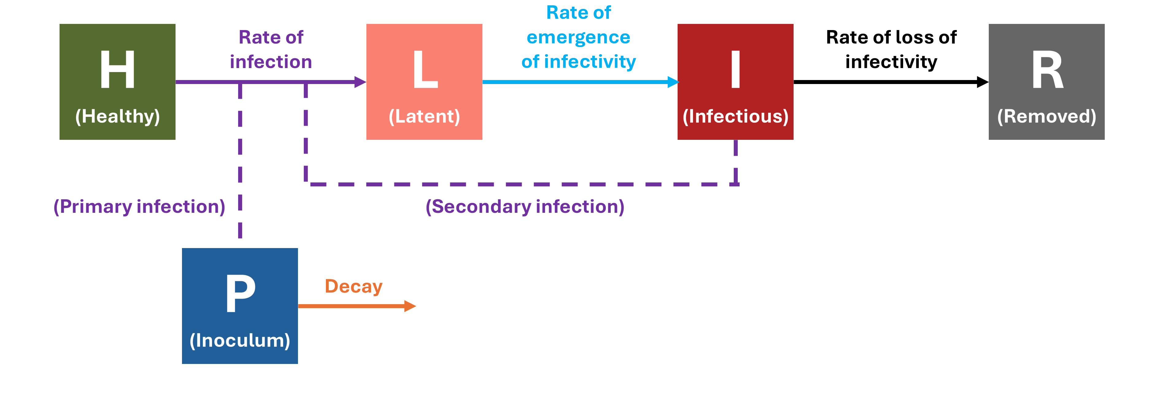
Schematic showing the H-L-I-R-(P) compartmental model. A new compartment has been added, which tracks the density of inoculum (i.e., this compartment does not relate to host status), which decays over time, but which infects healthy hosts. The two types of infection – primary and secondary – are distinguished on the diagram.

One way of doing this involves introducing an additional compartment, \(P\), which tracks the density of primary inoculum. We assume that primary inoculum only decays, but also leads to primary infection (and so a transition of hosts from \(H \rightarrow L\)). Primary infection is assumed to occur at a rate which is jointly proportional to the density of inoculum and the number of healthy hosts, i.e.,

\[\begin{aligned} \mbox{Net rate of primary infection} &\propto \mbox{Number of healthy hosts} \times \mbox{Density of inoculum}.\\ \end{aligned}\]

Note that there are now two infection pathways, the net result of which sets the overall rate of infection

  • Primary infection. Infection from outside the system (i.e., from the inoculum)
  • Secondary infection. Infection from within the system (i.e., from infectious hosts)

If we assume the inoculum (\(P\)) decays at characteristic rate \(\omega\) (per day per unit density of inoculum) and leads to primary infection at rate \(\alpha\) (per unit density of inoculum per healthy host), the equations of the H-L-I-R-(P) model are

\[\begin{aligned} \frac{dH}{dt} &= - \alpha P H - \beta I H ,\\ \frac{dL}{dt} &= \alpha P H + \beta I H - \gamma L,\\ \frac{dI}{dt} &= \gamma L - \mu I,\\ \frac{dR}{dt} &= \mu I,\\ \frac{dP}{dt} &= -\omega P. \end{aligned}\] This model can be simulated too.

Relative to our previous template, we need to

  • define a new function for the right hand side of the model
  • update the parameters to include \(\omega\) and \(\alpha\)
  • update the initial condition to include \(P(0)\)

Of course, numeric values for the two new parameters and one new initial condition are required. In the code below we set

  • \(\omega = 0.05\) day\(^{-1}\)
  • \(\alpha = 0.00001\) inoculum\(^{-1}\) day\(^{-1}\)
  • \(P(0) = 10\)

We also set

  • \(H(0) = 10000\)
  • \(L(0) = 0\)
  • \(I(0) = 0\)
  • \(R(0) = 0\)

which corresponds to assuming no hosts are infected at \(t=0\).

We have therefore assumed the inoculum has an average lifetime of \(1/\omega = 20\) days, and that there are \(10\) units of inoculum present at \(t = 0\).

The value of \(\alpha\) requires some interpretation. It is the infection rate of healthy hosts per unit inoculum per host per unit time. So, in a system with \(N=10000\) hosts, with \(P(0) = 10\), we would expect the initial net rate of primary infection to be \(N \alpha P(0) = 1\), and so for an average of one host to become infected via the primary infection pathway per day.

However, because the decay rate of inoculum is relatively large, this drops off quite rapidly (and is further reduced because as time goes by there are fewer healthy hosts to infect).

The code to simulate the model is given below. Note it is just a lightly edited version of the code we originally used to simulate the H-L-I-R model.

hlirp.model <- function(t, state, parameters) {
  with(as.list(c(state, parameters)), {
    dH <- - alpha * P * H - beta * I * H
    dL <- alpha * P * H + beta * I * H - gamma * L
    dI <- gamma * L - mu * I
    dR <- mu * I
    dP <- - omega * P
    list(c(dH, dL, dI, dR, dP))
  })
}


hlirp.params <- hlir.params
hlirp.params[["omega"]] <- 0.05
hlirp.params[["alpha"]] <- 0.00001

hlirp.init <- c(H = N, 
               L = 0, 
               I = 0, 
               R = 0,
               P = 10)

hlirp.time <- hlir.time

# Solve the model
hlirp.sol <- ode(y = hlirp.init, 
                 times = hlirp.time, 
                 func = hlirp.model, 
                 parms = hlirp.params)

# Cast results to a R data frame
hlirp.sol.df <- data.frame(hlirp.sol)

# Plot results using our custom helper function
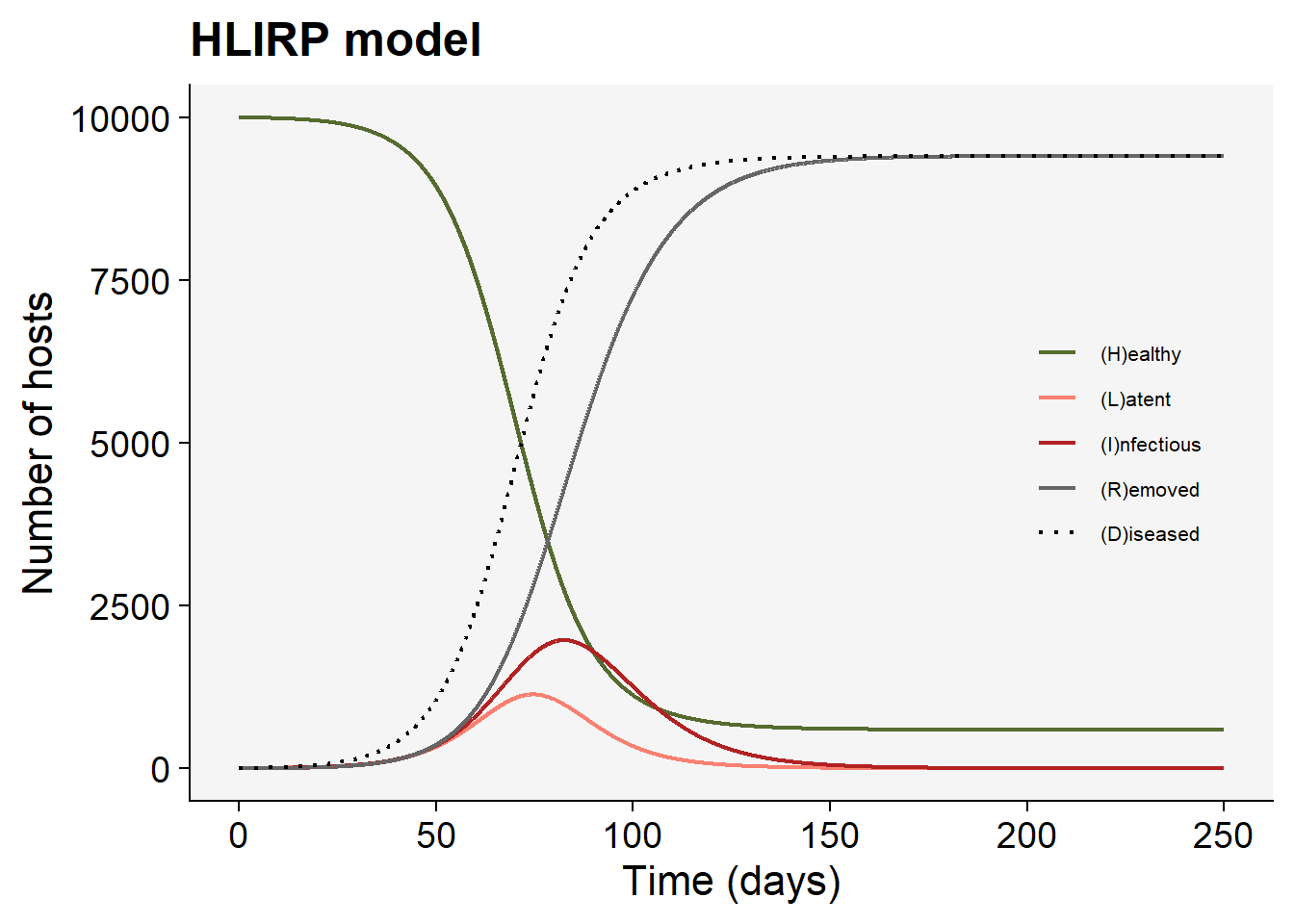
plot.model.results(hlirp.sol.df, type="HLIRP")

Compared with the previous simulation, primary inoculum removes the need for initial infected hosts, allowing the epidemic to start even when \(L(0)=I(0)=R(0)=0\).

Note that for these parameters, the epidemic gets going slightly more rapidly.

This formulation is useful not only for representing infection from outside the focal population, but also because it provides a mechanism by which inoculum carried over from one season can seed infection in the next (see below).

12.4.2 Adding host growth

Allowing host demography changes the balance between infection and replenishment, potentially altering both the growth rate and long-term behaviour of the epidemic.

We switch focus here, and focus on a crop plant host, which produces more infectable tissue over the course of the growing season (e.g., a wheat plant producing more leaves over time). It then makes sense to imagine the amount of host tissue being subject to its own dynamics, with an increase in the amount of tissue over time.

In what follows we will continue to refer to “hosts” for simplicity, even though now we are actually thinking about the number/density of infectable sites rather than whole plants.

There are various ways of modelling host growth. We introduce the idea in a simple way here, with logistic growth of healthy hosts at rate \(r_H\), to a carrying capacity \(N_{max}\). Adding this to the H-L-I-R-(P) model leads to \[\begin{aligned} \frac{dH}{dt} &= r_H H \left( 1 - \frac{H+L+I+R}{N_{max}}\right) - \alpha P H - \beta I H ,\\ \frac{dL}{dt} &= \alpha P H + \beta I H - \gamma L,\\ \frac{dI}{dt} &= \gamma L - \mu I,\\ \frac{dR}{dt} &= \mu I,\\ \frac{dP}{dt} &= -\omega P. \end{aligned}\] We have included the total amount of host tissue in the density-dependent term in the logistic growth, which corresponds to assuming all classes of host take up space and/or consume resources, whereas we have only included the number of units of healthy host in the production term. Depending on the system being modelled, it could, perhaps, be argued that \(R\) should be omitted from the density dependence, or \(L\) be included in the production term. It might also be appropriate to include natural exponential death terms on all state variables, to account for natural death of host tissue, but we have not done so here.

The updated model can again be solved by adapting our previous template. The following new parameter values are required

  • \(r_H = 0.05\) day\(^{-1}\)
  • \(N_{max} = 10000\)

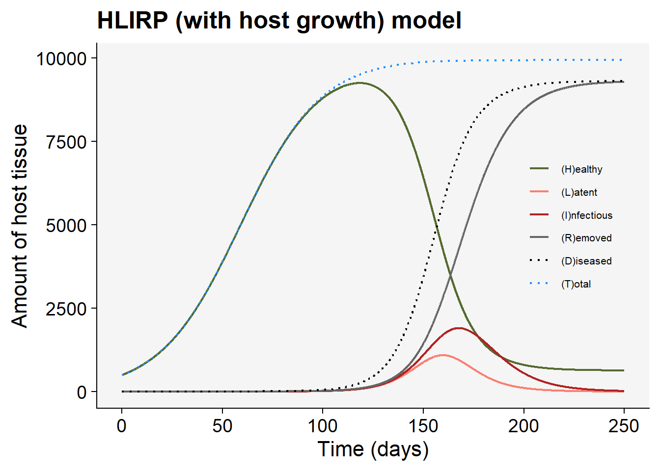
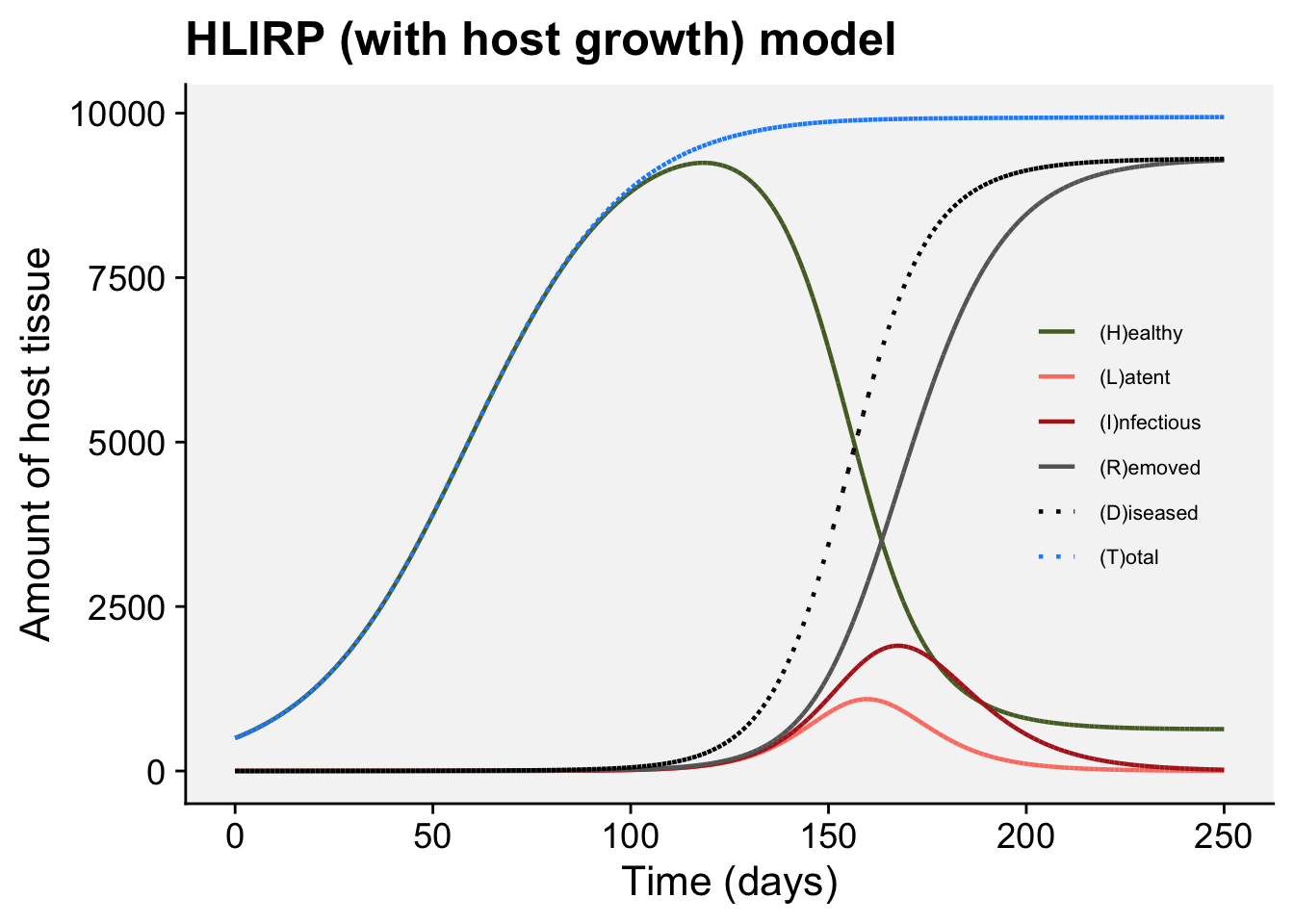
In the original H-L-I-R model, the total host population size was fixed, and we denoted this constant by \[N = H+L+I+R\] Once host growth is added, however, this quantity is no longer constant. To avoid confusion, we denote the time-varying total number of hosts by \[T(t) = H(t) + L(t) + I(t) + R(t).\] The carrying capacity for this total amount of host tissue is denoted by \(N_{\max}\). In the figure below, \(T(t)\) is shown by the dotted blue line. Also note that we start with \(H(0) = N_{max}/20\), i.e., a small number of hosts initially.

hlirp.with.growth.model <- function(t, state, parameters) {
  with(as.list(c(state, parameters)), {
    dH <- r.H * H * (1 - ((H + L + I + R)/N.max)) - alpha * P * H - beta * I * H
    dL <- alpha * P * H + beta * I * H - gamma * L
    dI <- gamma * L - mu * I
    dR <- mu * I
    dP <- - omega * P
    list(c(dH, dL, dI, dR, dP))
  })
}

hlirp.with.growth.params <- hlirp.params
hlirp.with.growth.params[["N.max"]] <- 10000
hlirp.with.growth.params[["r.H"]] <- 0.05

hlirp.with.growth.init <-  c(H = hlirp.with.growth.params[["N.max"]]/20, 
                             L = 0, 
                             I = 0, 
                             R = 0,
                             P = 10)

hlirp.with.growth.time <- hlir.time

# Solve the model
hlirp.with.growth.sol <- ode(y = hlirp.with.growth.init, 
                             times = hlirp.with.growth.time, 
                             func = hlirp.with.growth.model, 
                             parms = hlirp.with.growth.params)

# Cast results to a R data frame
hlirp.with.growth.sol.df <- data.frame(hlirp.with.growth.sol)

# Plot results using our custom helper function
plot.model.results(hlirp.with.growth.sol.df, type="HLIRP (with host growth)")

Note the epidemic is much slower and has only just completed by \(t = T_{max}\). This is because the epidemic only becomes self-sustaining when the amount of healthy host tissue is large enough that the effective reproduction number exceeds one. In this model, when infection is rare, a natural approximation to the instantaneous reproduction number is \(\beta H(t)/\mu\). Early in the season \(H(t)\) is low, so infection fails to increase even though host growth later creates enough healthy tissue for spread.

12.4.3 Accounting for multiple seasons

Extending the model across seasons introduces new mechanisms for persistence that are not captured by within-season quantities such as \(R_0\) alone.

12.4.3.1 Polyetic epidemics

A key distinguishing feature of crop disease epidemiology is the regular perturbations introduced by harvesting and replanting (Cunniffe et al. 2015a). Many crop disease epidemics are polyetic, unfolding over multiple growing seasons (Zadoks 1974). Obvious examples are diseases caused by soil-borne pathogens, or by other pathogens with long-lived survival structures. In yet other systems, an epidemic within the crop leads to infection of nearby volunteer plants or other vegetation, which serves as a natural reservoir of inoculum. In all of these systems, infection does not simply run its course and disappear within a single year; instead, inoculum produced in one season seeds epidemics in subsequent seasons.

We update our model to represent a polyetic crop epidemic over multiple growing seasons, again adding complexity gradually. This final model is loosely based on the models given in Sections 6.2.2 and 6.3 of the Madden et al. (2007) textbook, which themselves were based on the model presented in Madden and van den Bosch (2002).

However, we note there are many examples of models of polyetic epidemics in the plant disease modelling literature, ranging from models targeting biological control (Gubbins and Gilligan 1997), to fungicide resistance (Elderfield et al. 2018), to pathogen speciation (Hamelin et al. 2011), to integrated pest management (Vincent et al. 2025), to host plant resistance (Fabre et al. 2012), to fluctuations over years caused by stochastic emergence and re-emergence (Willocquet et al. 2020). All of these models of polyetic epidemics have the same fundamental ideas at their core; tracking the pathogen over successive growing seasons and modelling the process of inoculum carry-over from one season to the next.

12.4.3.2 Linking seasons via inoculum carryover

The H–L–I–R-(P) model as presented above implicitly describes a single-season epidemic. To extend this framework to multiple seasons, we must represent how infection or inoculum persists between seasons.

A simple way to represent multiple seasons is to assume that each season begins with a fresh population of healthy hosts, but with some carryover of infection pressure from the previous season via the inoculum compartment (\(P\)).

Let \(I_k(t)\) denote the time-dependent amount of infectious hosts during season \(k\). Within each season, the epidemic follows an H–L–I–R-(P) model, but the initial amount of inoculum depends on what happened in the previous season.

For example, we might assume:

  • a constant fraction of hosts are replanted at the start of each season, so \(H_k(0) = N_{max}/20\),
  • no hosts are actively infected at planting, so \(L_k(0) = I_k(0) = R_k(0) = 0\),
  • the initial amount of primary inoculum in season \(k\), \(P_k(0)\), depends on inoculum surviving from season \(k-1\).

A simple model of inoculum production and carryover between seasons is \[P_k(0) = \phi \int_0^{T_{max}} I_{k-1}(t)\,dt,\] where:

  • \(T_{max}\) is the length of the growing season,
  • \(\phi\) is rate at which infectious material is turned into inoculum (that survives between seasons).

Similarly to how we have treated host growth, more complex models of this component are possible, and here we have chosen to take a simple model that illustrates the underpinning idea.

The seasonal epidemic is represented by a continuous-time compartmental model, while the carry-over of inoculum is represented by a discrete-time map between seasons.

Within each season, the dynamics are as before, but the model must track the amount of inoculum produced. The following code introduces a function which does this using the results from the H-L-I-R-(P) model run above, doing the numerical integration via the function sfsmisc::integrate.xy.

library(sfsmisc)
Warning: package 'sfsmisc' was built under R version 4.4.3

Attaching package: 'sfsmisc'
The following object is masked from 'package:dplyr':

    last
find.inoc <- function(data, phi)
{
  inoc <- phi * integrate.xy(data$time,data$I)
  return(inoc)
}
phi <- 0.00001
print(find.inoc(hlirp.with.growth.sol.df, phi))
[1] 0.928291

12.4.3.3 Simulating multiple seasons

Having specified the mapping between successive seasons, the model is sufficiently “rich” to be able to track a multi-seasonal epidemic. We simulate over \(5\) years, starting from a very small initial amount of inoculum in season one, with \(P_1(0) = 0.0001\).

The top plot shows the amount of disease, \(D(t)\) and the total amount of host tissue, \(T(t)\) over successive seasons. The responses of the individual compartments (e.g., \(H(t),L(t),I(t)\) and \(R(t)\)) are not shown to avoid cluttering the figure.

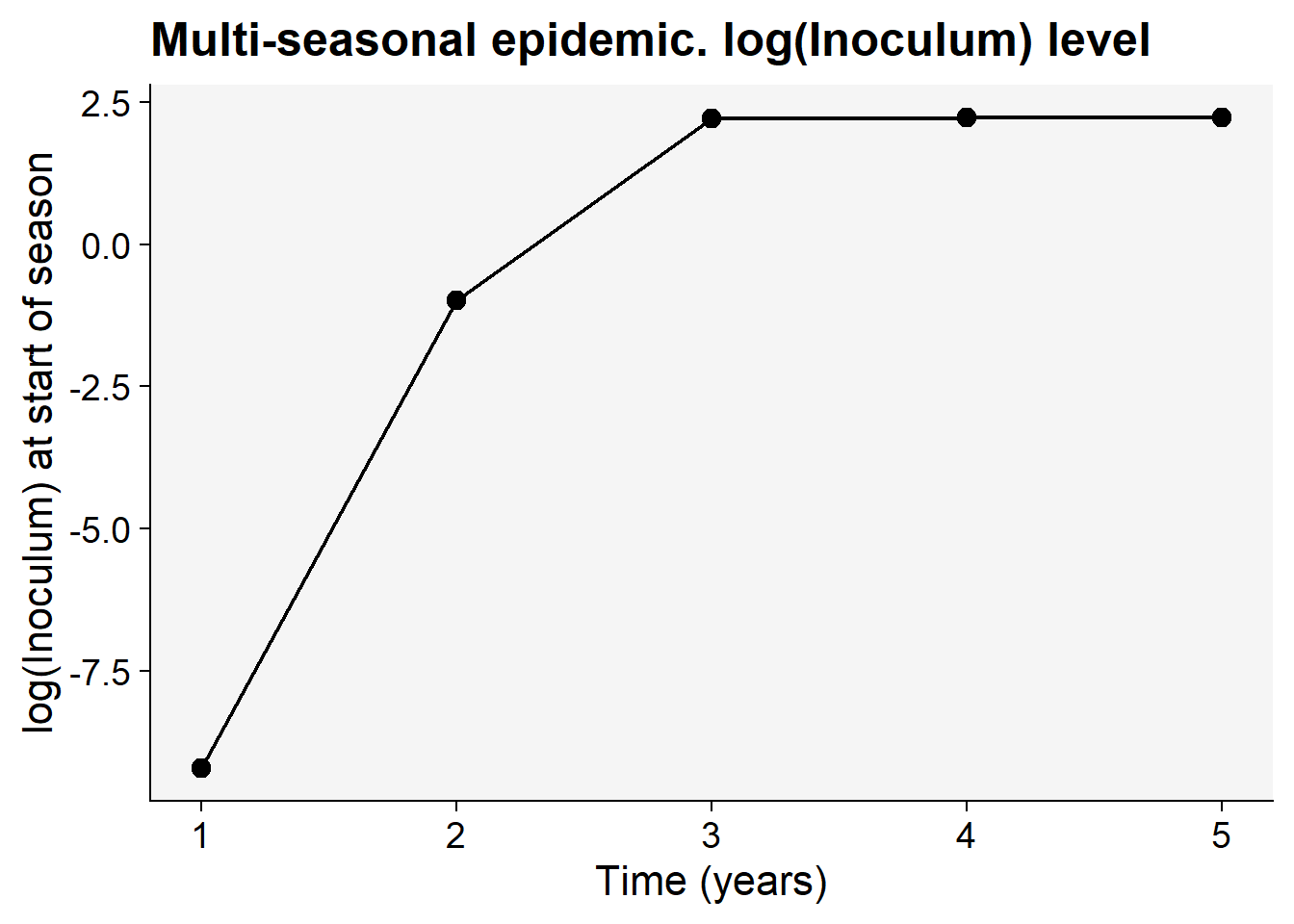
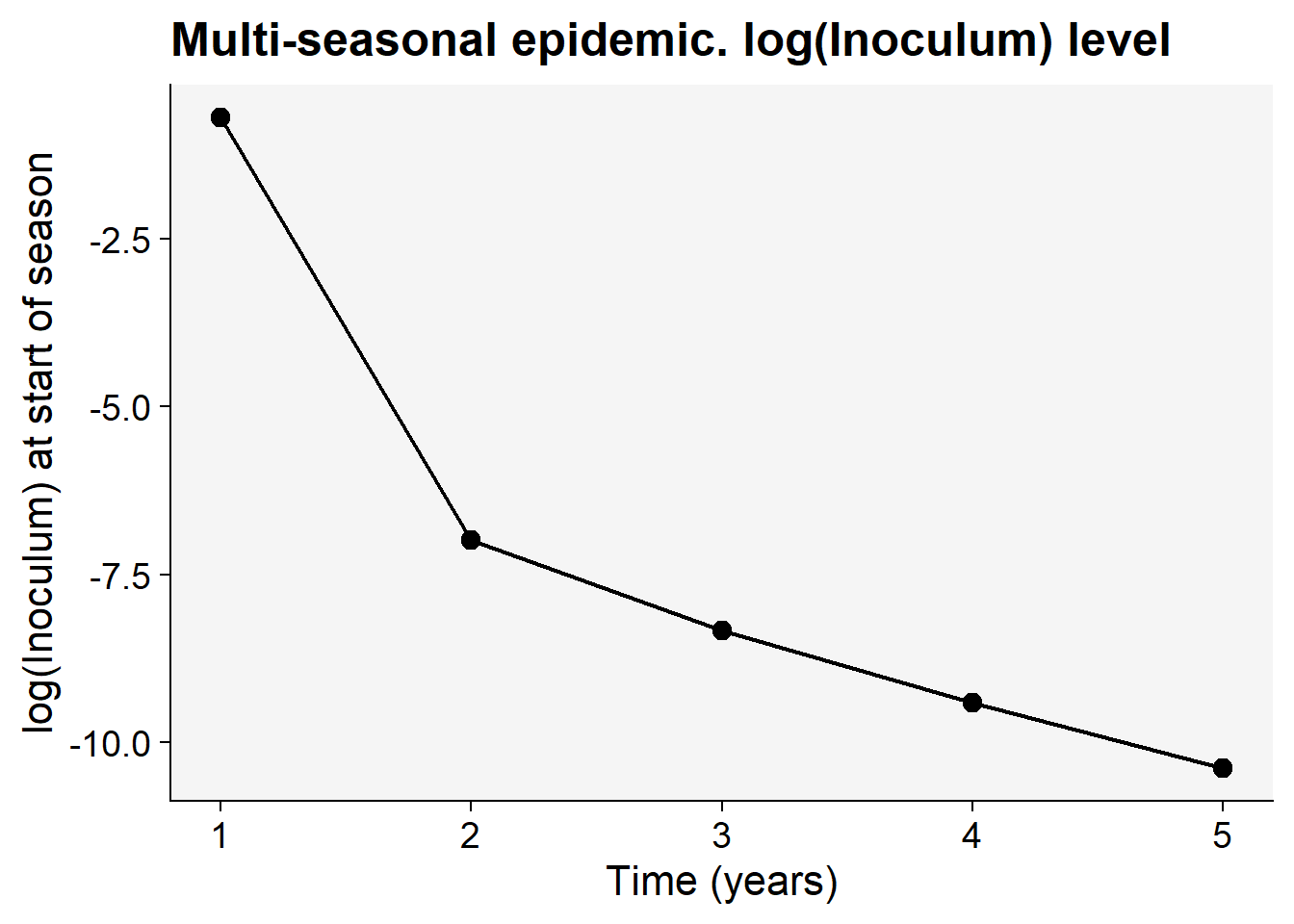
The bottom plot shows how the initial amount of inoculum, \(P_k(0)\) changes over time. This is shown on a logarithmic scale to allow small changes to be seen.

n.yr <- 5
init.inoc <- 0.0001
phi <- 1e-4
multi.to.plot <- list(n.yr = n.yr,
                      n.max = hlirp.with.growth.params[["N.max"]],
                      inoc = numeric(n.yr),
                      results = list())
for(i in 1:n.yr)
{
  # Update initial conditions
  hlirp.with.growth.init <-  c(H = hlirp.with.growth.params[["N.max"]]/20, 
                               L = 0, 
                               I = 0, 
                               R = 0,
                               P = init.inoc)
  # Store in the results structure
  multi.to.plot$inoc[i] <- init.inoc
  
  # Solve the differential equations
  hlirp.with.growth.sol <- ode(y = hlirp.with.growth.init, 
                               times = hlirp.with.growth.time, 
                               func = hlirp.with.growth.model, 
                               parms = hlirp.with.growth.params)
  
  # Cast results to a R data frame
  hlirp.with.growth.sol.df <- data.frame(hlirp.with.growth.sol)
  
  # Store in the results structure
  multi.to.plot$results[[i]] <- hlirp.with.growth.sol.df
  
  # Calculate how much inoculum was produced this season
  init.inoc <- find.inoc(hlirp.with.growth.sol.df, phi)
}
plot.model.results(multi.to.plot,"MULTI")

In the first year the small amount of inoculum leads to only a very small epidemic, although this does lead to a larger amount of inoculum at the start of year two. This then leads to a bigger epidemic, which produces an even larger amount of inoculum. After three years the system settles onto a repeated cycle, with the same amount of inoculum at the beginning of each year, and a correspondingly similar (and large) epidemic each year.

12.4.3.4 Epidemiological implications

The model including seasonality introduces new thresholds beyond the single-season basic reproduction number \(R_0\). In particular, even if there is a large epidemic within a season, if the carry over of inoculum between seasons is too small, the epidemic dies out.

This is illustrated below, in which the initial level of inoculum is much larger, but the production rate is much smaller (the code is omitted, which is identical apart from the values of the two parameters \(P_1(0)\) and \(\phi\)).

init.inoc <- 0.5
phi <- 1e-8

Over successive seasons the amount of inoculum becomes smaller, and the epidemic dies out. This is because the smaller value of \(\phi\) means that either less inoculum is produced within the season from a given amount of infectious tissue or that the inoculum is less good at surviving between seasons (these two mechanisms are not distinguishable within the current formulation of the model, although a more complex model could, of course, allow them to be disentangled).

12.5 Fitting to data

So far, compartmental models have been used to encode biological assumptions and to generate predictions about disease dynamics. In practice, however, epidemiological models are often used in the opposite direction: observations of disease are used to estimate unknown model parameters.

To illustrate the basic idea, we consider a simple example based on the H–L–I–R model. Suppose disease incidence has been measured through time during an epidemic and that all model parameters are known except the transmission rate, \(\beta\).

The goal is to use the observations to estimate the value of \(\beta\).

12.5.1 Generating a synthetic data set

To demonstrate the procedure, we first simulate an epidemic from the H-L-I-R model using a known value of \(\beta = 0.00002\) host\(^{-1}\) day\(^{-1}\). Note that the other parameters, as well as the initial conditions, are held fixed throughout; we are therefore only concentrating on estimating a single parameter.

We present a very simple treatment in which we assume all infected hosts – including latently infected hosts – are visible, and so would be scored as “diseased” in any experiment or field work. Of course, this could be challenged, and would definitely depend on the pathosystem of interest.

The key output of the model for fitting is therefore a set of values of \(D=L+I+R\) at particular times, \(t\).

Before fitting, we add a small amount of artificial noise to these “data”. For illustrative purposes, we add Gaussian noise whose variance is scaled to resemble that of a binomial process.

In the computational work hereafter, these observations are treated as if they were experimental data, and are used to estimate the value of the infection rate, \(\beta\).

library(deSolve)

find.dpc.hlir.known.beta <- function(this.beta,
                                     time.step = 20)
{
  this.hlir.params <- c(beta = this.beta, 
                        gamma = 0.2, 
                        mu = 0.1)
  
  # Specify initial conditions
  this.hlir.init <- c( H = 9999, 
                       L = 1, 
                       I = 0, 
                       R = 0)
  
  # Specify range of times for which a solution is required
  this.hlir.time <- seq(0, 250, by = time.step)
  
  # Solve the model
  this.hlir.sol <- ode(y = this.hlir.init, 
                       times = this.hlir.time, 
                       func = hlir.model, 
                       parms = this.hlir.params)
  
  # Cast results to a R data frame
  this.hlir.sol.df <- data.frame(this.hlir.sol)

  # Extract D = L + I + R and t
  dpc.data <- data.frame(time = this.hlir.sol.df$time,
                         D = this.hlir.sol.df$L + this.hlir.sol.df$I + this.hlir.sol.df$R)
  
  return(dpc.data)  
}

# seed the random number generator for replicability
set.seed(07072026)

true.beta <- 0.00002
this.N <- 10000

orig.dpc <- find.dpc.hlir.known.beta(true.beta)

p.disease <- orig.dpc$D / this.N
noise.sd <- sqrt(this.N * p.disease * (1 - p.disease))

orig.dpc$D.obs <- orig.dpc$D + 25 * noise.sd * rnorm(length(orig.dpc$D))
# truncate any out of range observations
orig.dpc$D.obs <- pmax(0, pmin(this.N, orig.dpc$D.obs))

12.5.2 Defining a measure of goodness of fit

To estimate \(\beta\) we need a measure of agreement between the model (for different values of \(\beta\)) and the observations.

A simple choice is the sum of squared errors, \[S(\beta) = \sum_i \left(D_{obs}(t_i) - D_{pred}(t_i; \beta)\right)^2\] where \(D_{obs}(t_i)\) is the observed amount of disease at time \(t_i\), and \(D_{pred}(t_i;\beta)\) is the corresponding model prediction for a particular value of \(\beta\).

The value of \(\beta\) that minimises \(S(\beta)\) is the best-fitting estimate of the transmission rate

find.ss.beta <- function(beta, data)
{
  this.dpc <- find.dpc.hlir.known.beta(beta)
  SS <- sum((this.dpc$D - data$D.obs)^2)
  return(SS)
}

12.5.3 Visualising the objective function

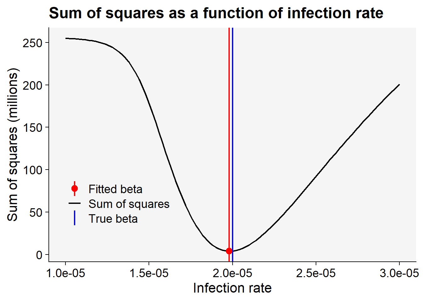
Before performing numerical optimisation, it is sensible to calculate \(SS(\beta)\) over a range of possible transmission rates, and to plot the results. Note that before plotting the y-value (the sum of squares) is divided by one million.

library(ggplot2)
library(r4pde)

all.beta <- seq(0.5 * true.beta, 
                1.5 * true.beta, 
                length.out = 101)
all.SS <- numeric(length(all.beta))
for(i in 1:length(all.beta))
{
  all.SS[i] <- find.ss.beta(all.beta[i],orig.dpc)
}
all.SS <- all.SS / 1000000

min_idx <- which.min(all.SS)
fitted_beta <- all.beta[min_idx]
min_ss <- all.SS[min_idx]

ss_df <- data.frame(
  beta = all.beta,
  ss = all.SS
)

p <- ggplot(ss_df, aes(x = beta, y = ss)) +
  geom_line(aes(color = "Sum of squares"), linewidth = 0.8) +
  geom_vline(aes(xintercept = true.beta, color = "True beta"), linewidth = 0.8) +
  geom_vline(aes(xintercept = fitted_beta, color = "Fitted beta"), linetype = "solid", linewidth = 0.8) +
  geom_point(data = data.frame(beta = fitted_beta, ss = min_ss), 
             aes(x = beta, y = ss, color = "Fitted beta"), size = 3) +
  scale_color_manual(
    values = c(
      "Sum of squares" = "black",
      "True beta" = "blue",
      "Fitted beta" = "red"
    )
  ) +
  labs(
    x = "Infection rate",
    y = "Sum of squares (millions)",
    title = "Sum of squares as a function of infection rate",
    color = NULL
  ) +
  theme_r4pde() +
  theme(legend.position = c(0.05, 0.25)) +
  guides(color = guide_legend(override.aes = list(linetype = "solid")))

print(p)

The sum of squares has a clear minimum. This is the value of \(\beta\) which has the closest match between model and observations.

The value has been obtained above by a one-way scan as

print(paste("Estimated beta (one way scan) =", all.beta[which.min(all.SS)]))
[1] "Estimated beta (one way scan) = 1.98e-05"

12.5.4 Numerical optimisation

Although the minimum can be identified visually, optimisation algorithms provide a more efficient and general approach. In the code below, this is done using the optim() function in R. This requires an initial guess at the optimal value of \(\beta\); it is set to be a random value within 50% of the true value.

fit <- optim(par = true.beta * runif(1,min=0.5,max=1.5), 
             fn = find.ss.beta,
             data = orig.dpc,
             method = "L-BFGS-B",
             lower = 0,
             control = list(parscale = 1e-5)) # note need last argument to 
                                              # avoid optimiser thinking it has
                                              # converged when it has not 
                                              # (due to large values of SS)

beta.hat <- fit$par

print(paste("Estimated beta (optim) =", beta.hat))
[1] "Estimated beta (optim) = 1.98176029764101e-05"

The parscale argument rescales the optimisation problem so that changes in \(\beta\) of order \(10^{-5}\) are treated as numerically meaningful by the optimiser.

The estimate of \(\beta\) is very close to the true value used to generate the synthetic data. In a real application, however, the true parameter value would of course be unknown.

12.5.5 Interpretation

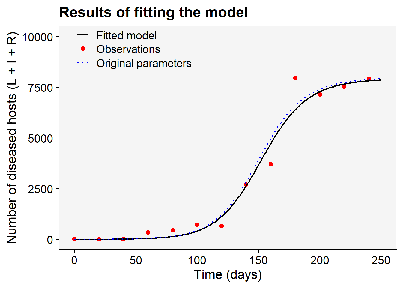
To assess the quality of the fit, the fitted model predictions can be plotted against the observations (see below).

library(ggplot2)
library(r4pde)

fitted.dpc <- find.dpc.hlir.known.beta(beta.hat, 
                                       time.step=1)

# recalculate the dpc for the original data set 
# to make the graph appear smoother
orig.beta.dpc <- find.dpc.hlir.known.beta(true.beta, 
                                          time.step=1)

p <- ggplot() +
  # Observations (points)
  geom_point(data = orig.dpc, aes(x = time, y = D.obs, color = "Observations"), size = 2) +
  # Fitted model (solid line)
  geom_line(data = fitted.dpc, aes(x = time, y = D, color = "Fitted model"), linewidth = 0.8) +
  # Original parameters (dashed line)
  geom_line(data = orig.beta.dpc, aes(x = time, y = D, color = "Original parameters"), linetype = "dotted", linewidth = 0.8) +
  scale_color_manual(
    values = c(
      "Observations" = "red",
      "Fitted model" = "black",
      "Original parameters" = "blue"
    )
  ) +
  labs(
    x = "Time (days)",
    y = "Number of diseased hosts (L + I + R)",
    title = "Results of fitting the model",
    color = NULL
  ) +
  xlim(0, 250) +
  ylim(0, 10000) +
  theme_r4pde() +
  theme(legend.position = c(0.05, 0.9))

print(p)

The fitted model performs very well.

12.5.6 Summary

This simple example illustrates a general feature of epidemiological modelling: model parameters can be estimated by comparing the degree of concordance between observations and predictions. In practice we usually want confidence intervals rather than only point estimates, but the above shows the basic idea of how parameters can be estimated from disease progress data.

Although only a single parameter was estimated here, the same principles extend to more realistic applications. In practice, several parameters may be unknown simultaneously, data may be noisy or incomplete, and different combinations of parameter values may produce very similar epidemic trajectories. This final issue is known as parameter identifiability (Cunniffe et al. 2024). Consequently, determining which parameters can be reliably estimated from a given dataset is often an important modelling challenge in its own right.

More sophisticated approaches, including likelihood-based and Bayesian methods, are widely used in modern epidemiology. Nevertheless, the underlying principle remains the same: parameters are estimated by identifying the model that best explains the observed data.

12.6 Further extensions

The H–L–I–R framework provides a useful and biologically interpretable starting point for modelling plant disease epidemics. However, the assumptions underpinning the model are often simplifications.

In the above, we have shown here how some of these assumptions can be relaxed. However, many applications require extensions that relax one or more of these assumptions. Important extensions include:

  • Multiple strains, allowing investigation of competition, coexistence and evolutionary change. Examples of models in the literature tracking multiple pathogen strains include Elderfield et al. (2018), Allen et al. (2019), Hamelin et al. (2019) and Taylor and Cunniffe (2023).
  • Multiple hosts, allowing investigation of pathosystems in which more than one host or variety of host can become infected. Examples include Bussell and Cunniffe (2022), Murray-Watson and Cunniffe (2023) and Del Ponte et al. (2026).
  • Vector-borne transmission, where insect vectors must be modelled alongside host populations. Examples include Donnelly et al. (2019), Cunniffe et al. (2021), Zaffaroni et al. (2021) and Falla and Cunniffe (2026).
  • Spatial structure, ranging from individual based models to patch-based models to explicit representations of pathogen dispersal across landscapes. Examples include Cunniffe et al. (2015b), Cunniffe et al. (2016), Hyatt-Twynam et al. (2017) and Ellis et al. (2025).
  • Stochastic dynamics, which capture chance events during invasion, extinction and disease persistence. Examples include Thompson et al. (2020), Fabre et al. (2021) and Russell and Cunniffe (2025).
  • Inference from data, where compartmental models are linked to observations to estimate parameters and quantify uncertainty. Examples include Gibson and Austin (1996), Adrakey et al. (2017), Thompson et al. (2018) and Best and Cunniffe (2026).

Although these extensions increase biological realism, they also introduce additional parameters, data requirements and computational complexity. Nevertheless, they retain the central idea introduced in this chapter: representing disease processes through biologically meaningful compartments and flows between them.

12.7 Summary

Compartmental models are probably best viewed as a flexible framework rather than a single model. A major strength of the framework is that additional biological complexity can often be incorporated simply by introducing new compartments or modifying transition rates. Starting from simple formulations, additional biological realism can be introduced in targeted ways to reflect specific epidemiological settings. The key challenge is not to maximise complexity, but to identify the simplest model that captures the dominant processes governing the epidemic. This principle underlies much of modern infectious disease modelling, irrespective of whether pathogen infecting plants, humans or animals are being considered. Throughout, the same framework serves three complementary purposes: representing biological mechanisms, understanding epidemic behaviour and extracting information from data.

12.8 Appendix. Relationship to population dynamics models

It is useful to show how simpler population dynamics models (as covered in Chapter 10) arise as limiting cases of the compartmental modelling framework.

We start with the H-L-I-R-(P) model (without host growth).

Assume that inoculum does not decay, i.e., \(\omega = 0\). This means the density of inoculum is fixed at \(P(0)\) for the whole epidemic, and the equation for \(dP/dt\) can be omitted.

Introduce the symbol \(\epsilon = \alpha P(0)\) to represent the fixed rate of primary infection (per healthy host) throughout the epidemic.

The H-L-I-R-(P) model then becomes

\[\begin{aligned} \frac{dH}{dt} &= -\left(\epsilon + \beta I\right) H,\\ \frac{dL}{dt} &= \left(\epsilon + \beta I\right) H - \gamma L,\\ \frac{dI}{dt} &= \gamma L - \mu I,\\ \frac{dR}{dt} &= \mu I. \end{aligned}\]

Assume that the latent period is infinitesimally short (i.e., \(\gamma \rightarrow \infty\)) and that infectious tissue does not lose infectivity (i.e., \(\mu = 0\)). This simplifies the dynamics \[\begin{aligned} \frac{dH}{dt} &= -\left(\epsilon + \beta I\right) H,\\ \frac{dI}{dt} &= \left(\epsilon + \beta I\right) H.\\ \end{aligned}\] But then, since \(H + I = N\), the model reduces down to a single equation for the number of infected plants \[ \frac{dI}{dt} = \left(\epsilon +\beta I\right)(N-I).\\\] As a historical aside, note this form of model was introduced by Brasset and Gilligan (1988) as a “differential equation that combines the properties of the monomolecular and logistic models”, and used to understand take-all disease in wheat. Here we have seen how it can be derived from the H-L-I-R model.

Recall the simpler population dynamics models are normally phrased in terms of the proportion of diseased plants/tissue. As described near the start of this chapter, this can be done here by considering \(y = I/N\), which leads to \[ \frac{dy}{dt} = \left(\epsilon+\beta N y \right)(1 - y),\\\]

12.8.1 Logistic model

The logistic model is \[\frac{dy}{dt} = r_L y(1-y),\] in which \(r_L\) is the rate parameter. The solution is \[y = \frac{1}{1 + \left(\frac{1-y_0}{y_0} \right)\exp(-r_L t)},\] where \(y_0\) is the initial proportion of disease.

This is equivalent to the H-L-I-R-(P) model in the limit \(\epsilon \rightarrow 0\), i.e., when there is no primary infection, and with the parameter identification \(\beta N = r_L\).

12.8.2 Monomolecular model

The monomolecular model is \[\frac{dy}{dt} = r_M (1-y),\] in which \(r_M\) is the rate parameter. The solution is \[y = 1 - (1 - y_0)\exp(-r_M t)\] where \(y_0\) is the initial proportion of disease.

This is equivalent to the H-L-I-R-(P) model in the limit \(\beta \rightarrow 0\), i.e., when there is no secondary infection, and with the parameter identification \(\epsilon = r_M\).

12.8.3 Exponential model

The exponential model is \[\frac{dy}{dt} = r_E y,\] in which \(r_E\) is the rate parameter. The solution is \[y = y_0\exp(r_E t)\] where \(y_0\) is the initial proportion of disease.

This is equivalent to the H-L-I-R-(P) model in the limit \(\epsilon \rightarrow 0\) and \(y \approx 0\), i.e., the exponential model is recovered when there is no primary infection and when \(y\) remains small, with the parameter identification \(\beta N = r_E\) \[ \frac{dy}{dt} \approx \beta N y.\]

12.8.4 Gompertz model

A concordance between process-based models and the Gompertz model can be made if we move to a more complex Kermack-McMcKermack type model in which the infection rate depends on the time-since-infection (Cunniffe et al. 2012; Segarra et al. 2001), at least approximately. However, this is really quite advanced and requires going well beyond what can be covered in this chapter, so we do not pursue this here.